Notes by Lex Toumbourou

• Ideas from computer vision are bleeding into other fields: speech recognition, NLP etc.
• Domains:
  • Image classification.
  • Object detection (self driving cars detecting other cars).
  • Neural style transfer.
• Challenge of computer vision: input sizes can get big.
  • 1000 x 1000 x 3 = 3M (3 megapixels)

Edge detection example

• Given an image, the computer may do object detection using vertical edges and horizontal images. How would one approach it?
• Take a 3x3 "filter" and perform a "convolution" operation.

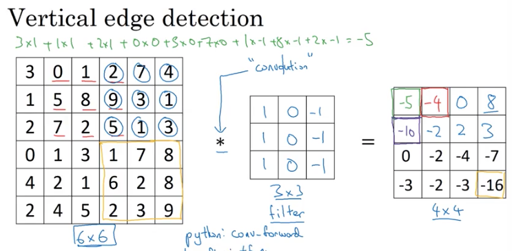
• Basically place the filter over a 3x3 section of an input image and take the element-wise product every place you can.
  • Research papers may call a filter a "kernel".
  • Output of convolution for a 6x6 input, would be a 4x4 matrix. Output can be thought of as an image.
• Most frameworks have functions for implementing convolution operations.

More edge detection

• Vertical edge detector:

[1, 0, -1] [1, 0, -1] [1, 0, -1]

• Horizontal edge detector:

[ 1, 1, 1] [ 0, 0, 0] [-1, -1, -1]

• Other filters:

  • Sobel filter (more weight to central pixel)

  [1, 0, -1] [2, 0, -2] [1, 0, -1]

  • Scharr filter

  [ 3, 0, -3] [10, 0, -10] [ 3, 0, -3]

• Constructing the filter can also be presented as an optimisation problem, where we use backprop to attempt to find the optimimal filters for the problem.

Padding

• If you take 6x6 input, convolv with a 3x3 filter, you end up with a 4x4 output matrix. That's a problem because:
  • Do it enough times, you end up a 1x1 image (shrinking output).
  • Pixels in the corner are used a lot less in the output.
  • If image is n x n and filter is f x f, the output size is: n - f + 1
    • 6 x 6 input, 3 x 3 filter = 6 - 3 + 1 = 4.
• Solution: add zero padding around the edges to ensure the output image is the same size as input (6x6 becomes 8x8).
  • In that example, p=1 because you're adding 1 layer of padding to every edge.
  • New formula: n + 2p - f + 1 = output
    • 6 + 2 - 3 + 1 = 6
• Two common choices for padding:
  • "Valid": no padding.
  • "Same": output image is same size as input.
  • p = (f-1) / 2
• f is usually odd in computer vision.
  • Allows for padding the same dimension all the way around.
  • Nice to have a central pixel in the filter.

Strided Convolutions

• Instead of moving filter one pixel for each conv calculation, you do it n pixels, where n is the "stride size".
• Output size is: floor($\frac{n + 2p - f}{s} + 1$) x floor($\frac{n + 2p - f}{s} + 1$)
• Math textbooks generally perform another operation on the filter by flipping it on the horizontal and vertical axis:

[ 3, 4, 5] [ 1, 0, 2] [-1, 9, 7]

=

[ 7, 2, 5] [ 9, 0, 4] [-1, 1, 3]

• Math mathematicians would call the deep learning convolution operation: "cross correlation".
• Generally the mirroring operation is ignored in deep learning literature.

Convolutions over volume

• Input has dimensions: 6 x 6 x 3 (where 3 is the number of channels).
• Filter also has a dimension for channels (that must match the input): 3 x 3 x 3.
• Conv output doesn't include the channel: 4 x 4.
• To calculate a conv in dimensions, you place the first filter block channel over the first channel of the input, then the second and then the third and add all results together to create a single block in the output conv.
• You could have a filter that is only interested in edge detection for certain colours.
• What if you wanted to use multiple filters (eg detecting vertical and horizontal edges etc)?
  • Can create multiple filters and create multiple outputs. Output dimensions become 4 x 4 x o where o is number of filters.
• Summary: n x n x nc * f x f x nc -> ((n - f + 1) / 4) * (n - f + 1) / 4) * nc
• Number of channels is also called "depth" in deep learning literature.

One layer of a convolutional network

• Add bias to output image and apply a non-linearity function (like relu).
• If you have 10 filters that are 3 x 3 x 3 in one layer of a neural network, how many params does the layer have?
  • Each filter has 27 (3x3x3) params + a bias (+1), so 28 params.
  • With 10 of them, you have 280.
  • Image size doesn't affect the number of parameters.
• Summary of notation:
  • $f^{[l]} = \text{filter size}$
  • $p^{[l]} = \text{padding}$
  • $s^{[l]} = \text{stride}$
  • $\text{Input}: n_H^{[l-1]} * n_W{[l-1]} * n_c^{[l-1]}$
  • $\text{Output}: n_H^{[l]} * n_W^{[l]} * n_C^{[l]}$
  • $N^H{[l]} = \frac{n_H^{[l-1]} + 2p^{[l]} - f^{[l]}}{s^{[l]}} + 1$

Pooling Layers

• Used to reduce size of representation to speed up computation and make features detected more robust.
• Max pooling: for a x by x region, take the max of each pixel.
• Introduces hyperparameters f and s:
  • f: size of pool (f=2 would be a 2x2 pool).
  • s: pool stride (number of blocks to skip over when finding pools).
• 3d input would perform pooling computations on each channel, ending up with an output shape with the same number of channels.
• Average pooling: instead of taking maxes within each pool, take the average.
  • Max pooling is more common than average.
  • Might use average pooling to collapse representation on a very deep nn.
• Can use padding with max pooling but it's very uncommon.
• Pool is performed for each channel.
• No parameters to learn with max pooling: all hyperparameters set by hand.

Why convolutions?

• Two main advantages over FC layers:

  1. Parameter sharing.
  2. Sparsity of connections.

• If you had an image that was 32x32x3 in size, with 6 5x5 filter to result in a 28x28x6 output, you'd need:

3072 * 4704 ~ 14M

params (a lot!)

• Parameter sharing
  • a filter that's useful in one part of the image, may be useful in another.
  • each feature detector can use the same parameters in a lot of different positions, thus reducing parameters.
• Sparsity of connections: in each layer, each output only depends on a small number of inputs.
  • Allows for training for smaller dataset.
  • Less chance of overfitting.
• Conv structure helps with translation invariance (a cat in the top left corner or bottom left corner is still a cat).