Week 3 - Object detection
Object localization
- Localization and detection:
- Image classification:
- Figuring out what an image is.
- Output a class label.
- Usually one object.
- Classification with localization
- Figure out what an image is and put a bounding box around the thing.
- Output a class label plus bounding box coordinates.
- Usually one object.
- Detection
- Localizing multiple objects in a picture, potentially across different classes.
- Often multiple objects.
- Classification with localisation
- Extends upon standard image classification to include bounding box in output.
- Bounding box represented with 4 numbers:
- bx, by to represent the centre point of box.
- bw to represent the width (as ratio ie 0.7)
- bh to represent the height.
- Defining the target label y (for 3 class problem):
- Pc = probability that there's an object (output 0 if no object).
- bx = centre point x coord.
- by = centre point y coord.
- bh = height.
- bw = width.
- c1 = is it class 1?
- c2 = is it class 2?
- c3 = is it class 3?
-
Loss function when Pc = 1 can be sum of squares of all elements:
- (noting that there are 8 output labels)
- When Pc = 0:
- because you don't care about the other values
- In practise, would use a log likelihood loss for c1, c2, c3 and squared error for bounding box coords.
Landmark Detection
- Model outputs x and y coords of important places: corner of eye, centre of nose etc.
- Building blocks of recognising emotions and things like snapchat filters.
- Requires big annotated training set.
Object Detection
- Creating car detection algorithm:
- Create dataset with closely cropped cars (either 1 (is car) or 0 (isn't car)) and train a model.
- Create a rectangle that slides across the image, for each rectangle feed to convnet to determine if it is or isn't a car.
-
Run multiple times with various different rectangle sizes.
-
Bigger stride == lower computational cost, worse performance.
- Lower stride == high computational cost, better performance (more chance of sliding across target object).
Convolutional Implementation of Sliding Windows
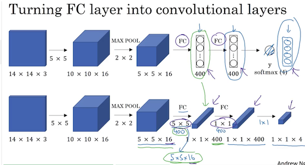
- Can convert the fully connected final layers of a standard conv model to conv layers as follows:
- Replace the second last fully connected layer, with 400 5x5 conv filters to return a 1x1x400 volume.
- Replace the last fc layer with a 1x1x400 conv layer.
- Replace the softmax output with a 1x1x4 conv layer.

- This conversion lets you implement a convolutional implementation of sliding windows detection.
- Instead of running forward prop on a bunch of different sections of the image, can run it just once with the filters sharing a lot of data.
- Bounding boxes are generally not that accurate.
Bounding Box Predictions
- Output accurate bounding boxes: YOLO algorithm.
- YOLO: You only look once.
- Place grid over image, like 19x19.
- For any object in the image, find the midpoint and assign the cell it falls in as the cell containing the object.
- Create labels
y = [pc, bx, by, bh, bw, c1, c2, c3]for each of the grid cells as labels for training.
- Total volume of output: 19x19x8 (19x19 grid cells with 8 output elements in each).
- Bounding box predictions will be relative to the grid it's in.
bxandbyshould be between 0 and 1.bhandbwcan be greater than 1, since an object bounding box can fall outside the box.
- Problem of multiple images in a cell to be addressed later.
Intersection Over Union

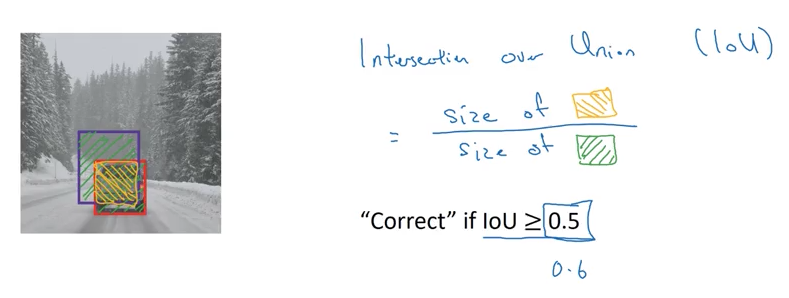
- Measure of overlap between 2 bounding boxes.
- Bounding boxes considered correct if IoU >= 0.5.
Non-max Suppression
- Because you are running the object classification and localization algo for every grid cell, it's possible you may end up with multiple bounding boxes.
- Non-max suppression basically finds the highest probability detection and removes (or "suppresses") the others. Details:
- Discard all bounding boxes with Pc < 0.6 (low probability).
- Pick the box with the highest Pc and output as a prediction.
- You figure out which bounding boxes are intended for the same objects by looking at all bounding boxes with IoU >= 0.5 then discard.
- When you have multiple objects in an image, you'd do non-max suppresses for each class detected in the image.
Anchor boxes
- Deals with the problems of multiple object centre points in an image.
- The y outputs now include 8 x number of possible objects in a cell (sometimes up to 5).
- Change previous algo to find an object midpoint and anchor box.
YOLO Algorithm
- Training set construction:
- If you have 3 classes, 2 anchor boxes per grid and 3x3 grid, y is
3 x 3 x 2 x 8.- 8 outputs = 1 probability of object + 4 bounding boxes + 3 class labels.
- For any grid cells with no object midpoint, probability would be 0 for both anchor boxes.
- For grid cells with an object midpoint, you'd have one of the anchor boxes probabilities set to 1.
- If you have 3 classes, 2 anchor boxes per grid and 3x3 grid, y is
- Outputting non-max supressed outputs:
- For each grid cell, get 2 predicted bounding boxes.
- Get rid of low probability predictions.
- For each class (pedestrian, car, motorcycle), use non-max supression to output final predictions.
Region Proposals
- Run a "segmentation algorithm" to find "blobs" that you can potentially run your classifier on.
- Should reduce the amount of positions you have to run your convnet on.
-
R-CNN:
- Propose regions.
- Classify proposed regions outputting label + bounding box.
-
Fast R-CNN:
- Propose regions.
- Use conv implementation of sliding windows to classify proposed regions.
-
Faster R-CNN:
- Use conv network to propose regions.
- Andrew thinks region proposal is interesting, but believes YOLO is a more promising direction for computer vision.