Notes by Lex Toumbourou

What are eigen-things?

What are eigenvalues and eigenvectors?

• "Eigen" is translated from German as "characteristic."
• "Eigenproblem" is about finding characteristic properties of something.

• Geometric interpretation of Eigenvector and Eigenvalue (00:45-04:22)

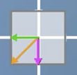
  • Though we typically visualize linear transformations based on how they affect a single vector, we can also consider how they affect every vector in the space by drawing a square.

    

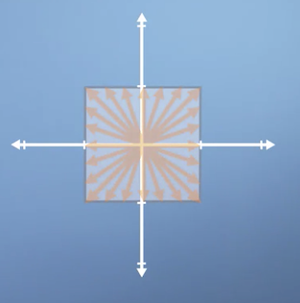
    We can then see how a transformation distorts the shape of the square.

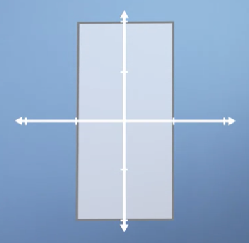
  • If we apply a scaling of 2 in vertical direction $\left( \begin{bmatrix}1 & 0 \\ 0 & 2\end{bmatrix} \right)$ the square becomes a rectangle.

    

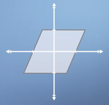
  • A horizontal sheer on the other hand looks like this: $\left( \begin{bmatrix}1 & s \\ 0 & 1\end{bmatrix} \right)$

    

  • When we perform these operations:

    • Some vectors point in the same direction but change length.
    • Some vectors point in a new direction.
    • Some vectors do not change.

    

  • The vectors that point in the same direction we refer to as Eigenvector.

  • The vectors that point in the same direction and whose size does not change are said to have Eigenvalues 1.
    • In the above example, the vertical Eigenvector doubles in length, with an Eigenvalue of 2.
  • In a pure sheer operation, only the horizontal vector is unchanged. So the transformation has 1 Eigenvector.
  • In a rotation, there are no Eigenvectors.

Getting into the detail of eigenproblems

Special eigen-cases

• Recap (00:00-00:18):
  • Eigenvector lie along the same span before and after applying a linear transform to a space.
  • Eigenvalues are the amount we stretch each of those vectors in the process.

• 3 special Eigen-cases (00:18-02:15)

  • Uniform scaling
    • Scale by the same amount in each direction.
    • All vectors are Eigenvectors.

  • 180° rotation

    • In regular rotation, there are no Eigenvectors. However, in 180° rotation, all vectors become Eigenvector pointing in the opposite direction.

      • Since they are pointing in the opposite direction, we say they have Eigenvalues of -1.

        

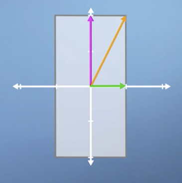
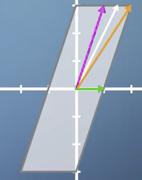
  • Combination of horizontal sheer and vertical scaling

    • Has 2 Eigenvector. The horizontal vector and a 2nd Eigenvector between the orange and pink vector.

      

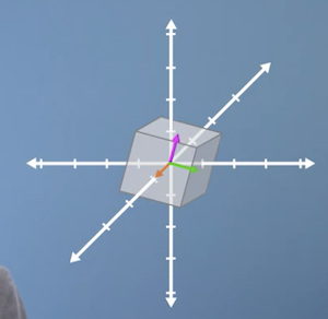
• We can calculate Eigenvalues in much higher dimensions.

  • In the 3d example, finding the Eigenvector also tells you the axis of rotation.

    

Calculating eigenvectors

• Calculating Eigenvector in general case (00:24-04:36)
  • Given transformation $A$, Eigenvectors stay on the same span after the transformation.
  • We can write the expression as $Ax = \lambda x$ where $\lambda$ is a scalar value, and $x$ is the Eigenvector.
  • Trying to find values of x that make the two sides equal.
    • Having A applied to them scales their length (or nothing, same as scaling by 1)
  • A is an n-dimensional transform.
  • To find the solution of the express, we can rewrite:
    • $(A - \lambda I)x = 0$
      • The $I$ is an $n \times n$ Identity Matrix that allows us to subtract a matrix by a scalar, which would otherwise not be defined.
    • For the left-hand side to be 0, either:
      • Contents of the bracket are 0.
      • x is 0
    • We are not interested in the 2nd case as it means it has no length or direction. We call it a "trivial solution."
    • We can test if a matrix operation results in 0 output by calculating its Matrix Determinate: $det(A - \lambda I) = 0$
    • We can apply it to an arbitrary 2x2 matrix: $A = \begin{bmatrix}a & b \\ c & d \end{bmatrix}$ as follows: $det(\begin{bmatrix}a & b \\ c & d \end{bmatrix} - \begin{bmatrix}\lambda & 0 \\ 0 & \lambda \end{bmatrix}) = 0$
    • Evaluating that gives us the Characteristic Polynomial: $\lambda^{2} - (a+d) \lambda + ad - bc = 0$
    • Our Eigenvalues are the solution to this equation. We can then plug the solutions into the original expression.
• Applying to a simple vertical scaling transformation (04:36-07:53):
  • Give vertical scaling matrix: $A = \begin{bmatrix}1 & 0 \\ 0 & 2\end{bmatrix}$
  • We calculate the determinate of $A - I\lambda$: $det \left( \begin{bmatrix}1 - \lambda & 0 \\ 0 & 2 - \lambda \end{bmatrix} \right)$ as $(1-\lambda)(2-\lambda)$ which equals $0$
  • This means our equation has solutions at $\lambda = 1$ and $\lambda = 2$.
  • We can sub these two values back in:
    • 1st case: $@\lambda = 1$: $\begin{bmatrix}1 & -1 & 0 \\ 0 & 2 & -1\end{bmatrix} \begin{bmatrix}x_1 \\ x_2\end{bmatrix} = \begin{bmatrix}0 & 0 \\0 & 1 \end{bmatrix}\begin{bmatrix}x_1 \\ x_2 \end{bmatrix} = \begin{bmatrix}0 \\ x_2\end{bmatrix} = 0$
    • 2nd case: $@\lambda = 2$: $\begin{bmatrix}1 & -2 & 0 \\ 0 & 2 & -2\end{bmatrix} \begin{bmatrix}x_1 \\ x_2\end{bmatrix} = \begin{bmatrix}-1 & 0 \\0 & 0 \end{bmatrix}\begin{bmatrix}x_1 \\ x_2 \end{bmatrix} = \begin{bmatrix}-x_1 \\ 0\end{bmatrix} = 0$
  • We know that any vectors that point along the horizontal axis can be Eigenvector of this system.
    • $@\lambda = 1$: $x=\begin{bmatrix}t \\ 0\end{bmatrix}$
      • When $\lambda=1$, the Eigenvector can point anywhere along the horizontal axis.
    • $@\lambda = 2$: $x=\begin{bmatrix}0 \\ t\end{bmatrix}$
      • When $\lambda=2$, the Eigenvector can point anywhere along the vertical axis.
• Applying to a 90° rotation transformation (07:54-)
  • Transformation: $A=\begin{bmatrix}0 & -1 \\ 1 & 0\end{bmatrix}$
  • Applying the formula gives us $\text{det}( \begin{bmatrix}0 - \lambda & -1 \\ 1 & 0-\lambda) \end{bmatrix} = \lambda^{2} + 1 = 0$
  • Which means there are no Eigenvectors.
    • Note that we could still calculate imaginary Eigenvectors using imaginary numbers.
• In practice, you never have to calculate Eigenvectors by hand.

When changing to the eigenbasis is useful

Changing to the eigenbasis

• Multiple matrix multiplications

  • Combines the idea of finding Eigenvector and changing basis.

  • Motivation:

    • Sometimes, we have to apply the same matrix multiplication many times.
    • For example, if you have a matrix that represents a change to a single particle after a specific timestep: $T = \left( \begin{bmatrix}0.9 & 0.8 \\ -1 & 0.35\end{bmatrix} \right)$ and you apply to a matrix $v_0 = \begin{bmatrix}0.5 \\ 1 \end{bmatrix}$ you end up with result: $v_1 = Tv_0$

    • You can apply it again to that result $v_2 = Tv_1$

      

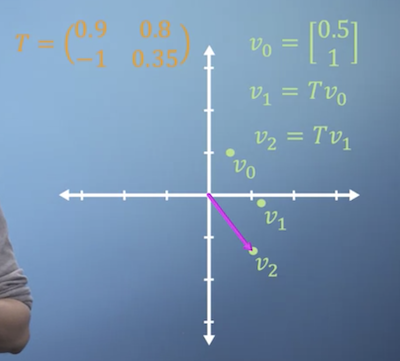
    • If you wanted to apply it millions of times, the operation could be expensive.

      • Can instead square $T$ to get the same result: $v_2 = {T^2} v_0$ or to the power of any $n$: $v_n = {T^n} v_0$
      • If T was is a Diagonal Matrices, where all terms along the leading diagonal are 0, you can simply square the non-zero values as: $T^{n} = \begin{bmatrix}a^n & 0 & 0 \\ 0 & b^n & 0 \\ 0 & 0 & c^n\end{bmatrix}$
      • When all terms except those along diagonal are 0.
      • If the matrix isn't diagonal, you can construct a Diagonal Matrix using Eigenanalysis.
    • Constructing a Diagonal Matrix
      • Plug in Eigenvectors as columns: $C = \begin{bmatrix}x_1 & x_2 & x_3 \\ . & . & . \\ . & . & . \\ . & . & .\end{bmatrix}$
      • Create a diagonal matrix from that: $D = \begin{bmatrix} \lambda_1 & 0 & 0 \\ 0 & \lambda_2 & 0 \\ 0 & 0 & \lambda_3 \end{bmatrix}$
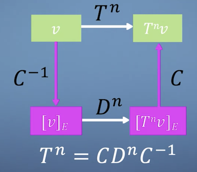
      • We then want to convert back to the original transformation, which we can use the inverse.
      • In summary: $T = CDC^{-1}$
      • Then $T^2$ would be: $T^{2} = CDC^{-1}CDC^{1}$
      • Since $C^1C$ returns the identity, we can rewrite as: $T^{n} = CD^{2}C^{1}$
    • The whole process looks like this:

  

Eigenbasis example

• Give a transformation matrix: $T = \begin{bmatrix}1 & 1 \\ 0 & 2\end{bmatrix}$
• When we multiply it with vector $\begin{bmatrix}1 \\ 0\end{bmatrix}$ the $\hat{i}$ vector is unchanged, so it's an Eigenvector with Eigenvalue 1.
• When multiplying with $\begin{bmatrix}1 \\ 1\end{bmatrix}$ gives us $\begin{bmatrix}2 \\ 2\end{bmatrix}$, so it's an Eigenvector with Eigenvalue 2.
• So, the Eigenvectors are:
  • $@\lambda = 1$: $n = \begin{bmatrix}1 \\ 0\end{bmatrix}$
  • $@\lambda = 2$: $n = \begin{bmatrix}1 \\ 1\end{bmatrix}$
• Transformation using squaring:
  • What happens to vector $\begin{bmatrix}-1 \\ 1\end{bmatrix}$ when you multiply it numerous times? $\begin{bmatrix}1 & 1 \\ 0 & 2\end{bmatrix}\begin{bmatrix}-1 \\ 1\end{bmatrix} = \begin{bmatrix}-1 + 1 \\ 0 + 2\end{bmatrix} = \begin{bmatrix}0 \\ 2\end{bmatrix}$ $\begin{bmatrix}1 & 1 \\ 0 & 2\end{bmatrix}\begin{bmatrix}0 \\ 2\end{bmatrix} = \begin{bmatrix}0 + 2 \\ 0 + 4\end{bmatrix} = \begin{bmatrix}2 \\ 4\end{bmatrix}$
  • If we instead started with $T^2$: $T^2 = \begin{bmatrix}1 & 1 \\ 0 & 2\end{bmatrix} \begin{bmatrix}1 & 1 \\ 0 & 2\end{bmatrix} = \begin{bmatrix}1 & 3 \\ 0 & 4\end{bmatrix}$ we can get straight to the answer: $\begin{bmatrix}1 & 3 \\ 0 & 4\end{bmatrix}\begin{bmatrix}-1 \\ 1\end{bmatrix} = \begin{bmatrix}2 \\ 4\end{bmatrix}$
• Transformation using Eigenbasis approach:
  • We have our conversion matrix from our Eigenvectors: $C = \begin{bmatrix}1 & 1 \\ 0 & 1\end{bmatrix}$
  • We know the inverse is: $C^{-1} = \begin{bmatrix}1 & -1 \\ 0 & 1\end{bmatrix}$
  • We can take the Eigenvalues to construct the diagonal matrix is $\begin{bmatrix}1 & 0 \\ 0 & 2\end{bmatrix}$
  • The problem is constructed as: $T^{2} = CD^2C^{-1} = \begin{bmatrix}1 & 1 \\ 0 & 1\end{bmatrix} \begin{bmatrix}1 & 1 \\ 0 & 2\end{bmatrix} \begin{bmatrix}1 & -1 \\ 0 & 1\end{bmatrix} = \begin{bmatrix}1 & 0 \\ 3 & 4\end{bmatrix}$
  • If we apply that to our original vector, we get the same results: $\begin{bmatrix}1 & 0 \\ 3 & 4\end{bmatrix}\begin{bmatrix}-1 \\ 1\end{bmatrix} = \begin{bmatrix}2 \\ 4\end{bmatrix}$

Making the PageRank algorithm

Introduction to PageRank

• PageRank (00:00-07:20)
  • Ranks websites by importance based on the importance of pages that link to them.
    • Central assumption: "the importance of a website is related it links to and from other websites."

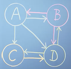
  • Model represents a model mini internet:

    

    • Network $1_A$ would have vector: $\begin{bmatrix}0 & 1 & 1 & 1\end{bmatrix}$ where a $1$ represents a link to it.
    • We then normalise the vector so the total probabilty sums to 1: $\begin{bmatrix}0 & 1/3 & 1/3 & 1/3 \end{bmatrix}$
    • Network $1_B$ would have vector: $\begin{bmatrix}1/2 & 0 & 0 & 1/2\end{bmatrix}$
    • Nework $1_C$: $\begin{bmatrix}0 & 0 & 0 & 1\end{bmatrix}$
    • Network $1_D$: $\begin{bmatrix}0 & 1/2 & 1/2 & 0\end{bmatrix}$
      • We can then convert each vector into a column of a matrix $L$: $\begin{bmatrix}0 & 1/2 & 0 & 0 \\ 1/3 & 0 & 0 & 1/2 \\ 1/3 & 0 & 0 & 1/2 \\ 1/3 & 1/2 & 1 & 0 \end{bmatrix}$
    • This matrix represents the probability of getting to each page. I.e., the only way to get to $A$ is from $B$.
    • You then need to know the probability of getting to $B$. You would need to be at either $A$ or $D$.
    • The problem is "self-referential": the ranks of all the pages depend on the ranks of others.
    • The columns are for external links, and the rows describe inward links normalized from the origin page.
      • An expression can be written using vector $r$ to store the rank of all web pages.
      • We can then get the rank for webpage A, as follows: $r_A = \sum\limits_{j=1}^{n} {L_A}_{j} r_j$
    • That means that the rank of $A$ is the sum of ranks of all pages that link to it, weighted by specific link probability taken from $L$.
      • We can rewrite that as simple matrix multiplication for all web pages: $r = Lr$
      • Since we start out not knowning $R$, we assume all ranks are equal and normalise by total webpages: $r=\begin{bmatrix}1/4 \\ 1/4 \\ 1/4 \\ 1/4\end{bmatrix}$
      • Then we keep updating iterative until $r$ stops changing: $r^{i+1}={L_r}^{i}$
      • Applying repeated means, we are solving iteratively until $r$ stops changing.
      • This means that $r$ is an Eigenvector of matrix $L$, with an Eigenvalue of 1.
    • We might assume that we could apply the Diagonalisation method, but we would first need to know all the Eigenvalues, which is what we're trying to find.
      • Though there are many approaches for efficiently calculating Eigenvectors, randomly multiplying a randomly selected initial guest vector by a matrix, called the Power Method, is still very effective.
    • The power method will only give you one Eigenvector for an n by n webpage system, the vector you get will be the one you're looking for with an Eigenvalue of 1.
    • The graph for the whole internet will be very Sparse Matrix. Algorithms exist that allow us to perform efficient matrix multiplication.
    • The damping factor $D$ (07:20-08:24)
      • Adds an additional term to formula: $r^{i+1}=d\left( {L_r}^{i} \right) + \frac{1-d}{n}$
      • It's the probability that a random web surfer will type a URL instead of clicking
      • Finds compromise between speed and stability.