Bias-Variance Tradeoff

A topic that a Machine Learning practitioner should know, if nothing else for the purposes of passing interviews, is the bias-variance trade-off.

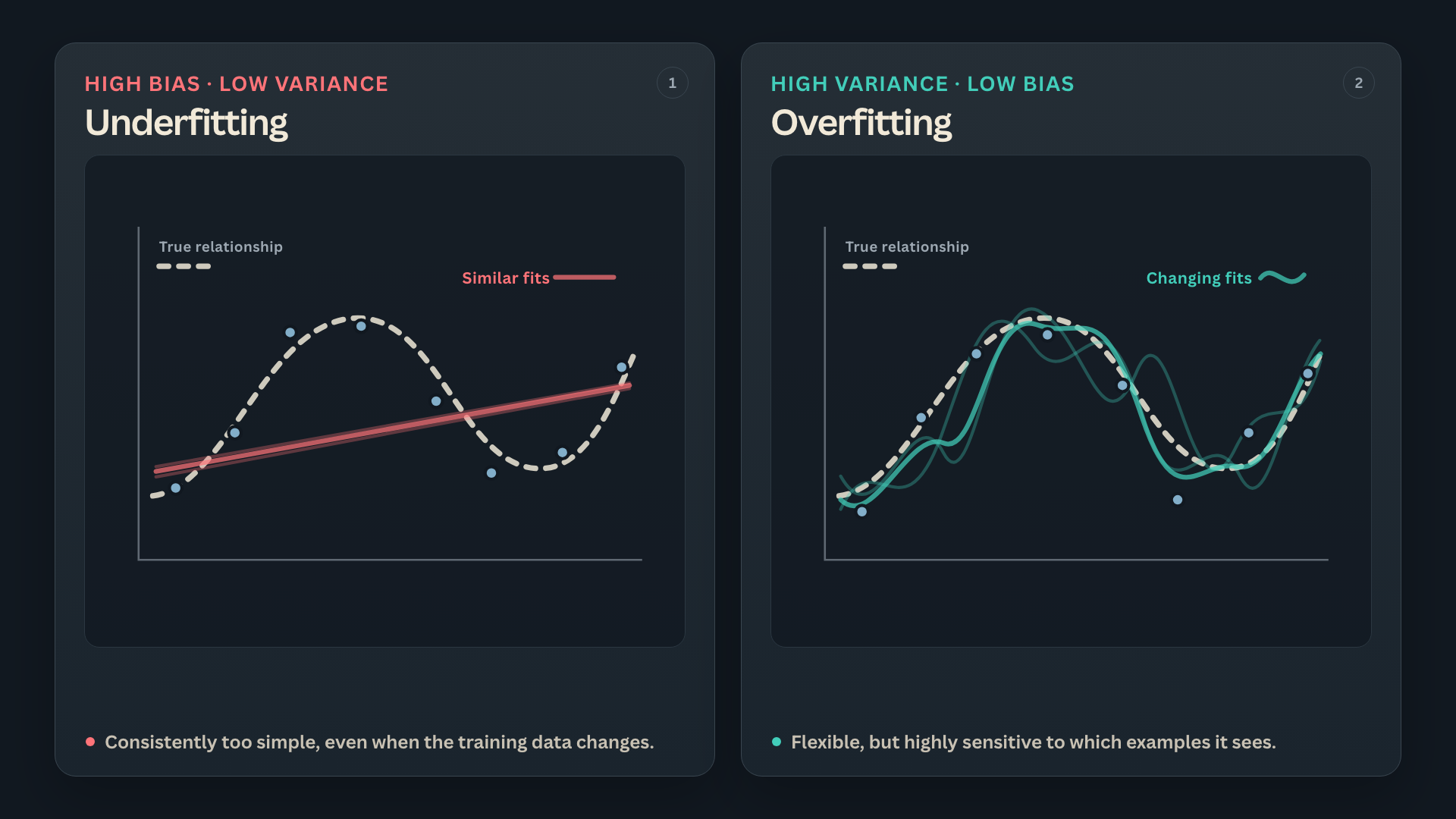
The basic idea is that simpler models tend to oversimplify the problem and fail to learn all the signal present in the data (underfitting). More complex models might fit the training data too closely and fail to generalise to new examples (overfitting).

The trade-off implies there is a level of model complexity that minimises expected test error by balancing bias and variance, as Fortmann-RoeScott (2012) shows:

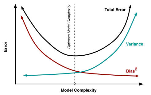
Note that the error here refers to Mean-Squared Error. Because MSE squares prediction errors, expanding its expected value produces a squared bias term.

---

Main thing to remember:

• High-Bias, Low-Variance is associated with underfitting
• High-Variance, Low-Bias is associated with overfitting

---

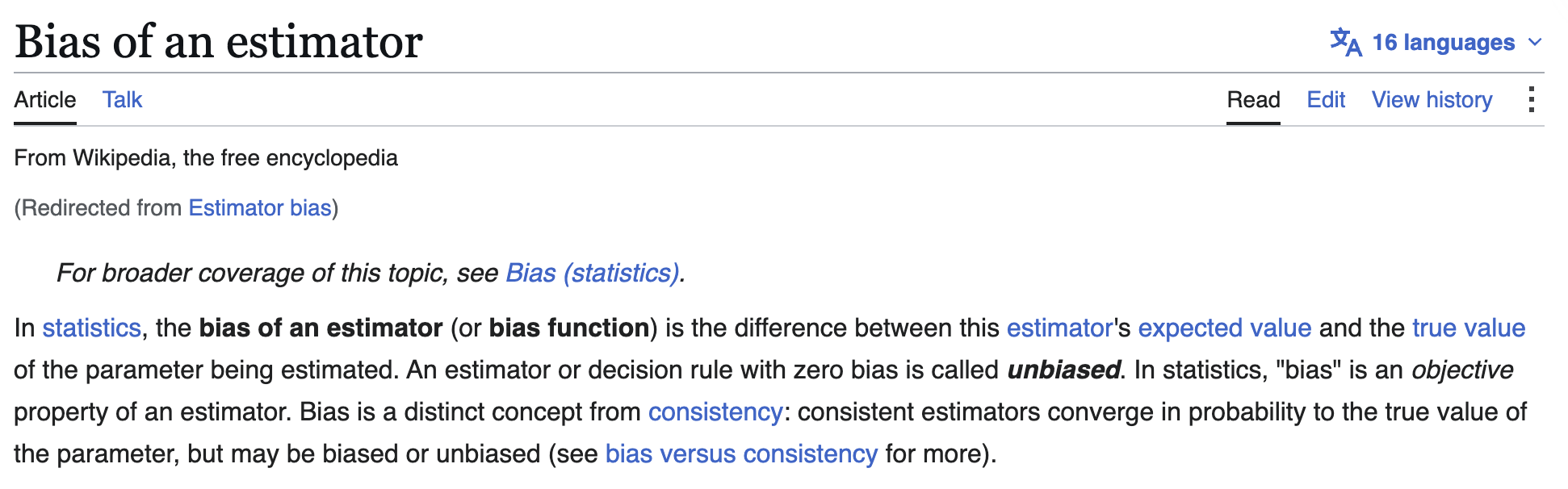
The word "bias" here comes from the statistical definition: the difference between a model's expected prediction across different training sets and the true value it's trying to estimate.

High bias is often introduced by a model that is too simple to accurately represent the problem.

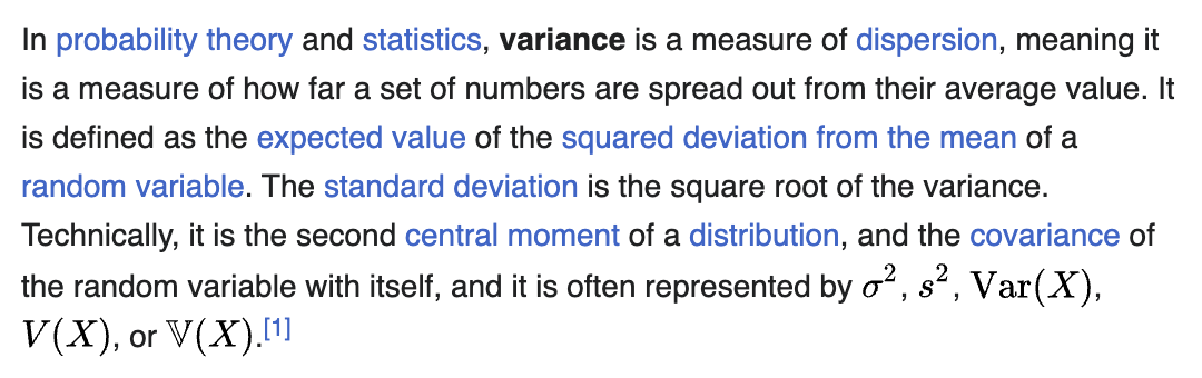
The word "variance" also comes from the statistical definition of variance: a measure of dispersion. The key idea is that it measures how far a model's predictions would be spread if you trained on different training datasets.

In the worst case, an extremely high-variance model may fit random noise in the training data - and not actually learn the things we care about.

---

This framing was applied to neural networks in the landmark work by Geman et al. (1992), but the idea goes back at least to Grenander's 1952 "uncertainty principle" in statistics (Grenander, 1952), with later examples in cubic smoothing splines and a 1990 statistics textbook (Neal, 2019).

In practice, the trade-off is seen as a fallacy - especially in the LLM era. There are many examples of complex models, especially neural networks, where increasing the size of the network can decrease both variance and bias (Neal, 2019).

Test error can also follow a double-descent curve: the classical U-shape is followed by a second descent after the model begins to interpolate the training data (Belkin et al., 2019).

Additionally, the kind of LLMs available today are constantly improving their ability to generalise to unseen tasks (or at least - the training sets are so big they encompass nearly everything we can think to test) - so it's not something you hear as much about.

Even so, there are still problems, especially with limited data, where the classical tradeoff is essential to understand.

---

Conventionally, to reduce bias, you might:

• use a more complex model (increase parameters, features, etc)
• reduce regularisation

Conversely, to reduce variance, you might:

• collect more data
• apply additional regularisation
• use a simpler model
• use data augmentation or early stopping
• combine multiple models through ensembling

---

For squared-error regression, the expected prediction error at a given $x$ is often decomposed as:

$MSE = \operatorname{Bias}(\hat{f}(x))^2 + \operatorname{Variance}(\hat{f}(x)) + \sigma^2$

Bias is squared because MSE measures squared error. Bias can be positive or negative, but either direction contributes to prediction error. When the expected squared error is expanded, the systematic difference between the model's expected prediction and the true value therefore appears as:

$\operatorname{Bias}(\hat{f}(x))^2 = \left(\mathbb{E}[\hat{f}(x)] - f(x)\right)^2$

This gives squared bias the same units as variance and MSE.

The term $\sigma^2$ represents the irreducible noise in the data that you cannot get rid of with a better model.

References

Mikhail Belkin, Daniel Hsu, Siyuan Ma, and Soumik Mandal. Reconciling modern machine-learning practice and the classical bias–variance trade-off. Proceedings of the National Academy of Sciences, 116(32):15849–15854, August 2019. doi:10.1073/pnas.1903070116. ↩

Stuart Geman, Elie Bienenstock, and René Doursat. Neural Networks and the Bias/Variance Dilemma. Neural Computation, 4(1):1–58, January 1992. doi:10.1162/neco.1992.4.1.1. ↩

Ulf Grenander. On empirical spectral analysis of stochastic processes. Arkiv för Matematik, 1(6):503–531, August 1952. doi:10.1007/BF02591360. ↩

Brady Neal. On the Bias-Variance Tradeoff: Textbooks Need an Update. December 2019. arXiv:1912.08286, doi:10.48550/arXiv.1912.08286. ↩ ^{1 2}

Fortmann-Roe, Scott. Understanding the Bias-Variance Tradeoff. https://scott.fortmann-roe.com/docs/BiasVariance.html, June 2012. ↩