Lesson 1: Recognizing Cats and Dogs¶

00:02:18 - Top-down vs bottom up¶

• Bottup-up: learn each building block then eventually put them together.
  • Traditional way stuff is taught.
  • Problems:
    • Hard to maintain motivation.
    • Hard to know the "big picture".
    • Hard to know which pieces you'll actually need.
• Top-down: learn by doing; slowly peal back the layers of the building blocks.
  • Fast.ai: start using neural net to get results straight away.

00:02:40 - GPUs¶

• Training neural network requires a GPU.
  • Requires an Nvidia GPU because they are the only ones that support CUDA.
• Renting GPUs:
  • Crestle (00:04:12)
    • Easiest.
    • Instant.
    • Provides access to only Jupyter Notebooks, not servers.
  • Paperspace (00:06:20)
    • Doesn't run on top of Amazon.
    • Provides their own virtual machines.
• Instructions on how to setup Paperspace (00:06:30)
  • Choose region.
  • Choose OS (Ubuntu 16.04)
  • Choose GPU+ (only 0.40 an hour)
    • Choosing a 0.65 / hr machine may require you to contact Paperspace to say why you're using it. Just say "Fast.AI".
  • To configure machine for course, log into terminal and type: curl http://files.fast.ai/setup/paperspace | bash
    • After running, need to restart Paperspace machine.
• Directory layout:
  • anaconda3
  • fastai
    • Course project directory.
• To start notebook:
  • cd into fastai directory and type juypter notebook.
  • Open lesson1.ipynb

00:13:00 - Jupyter instructions¶

• To run a cell: select the cell and hold down shift and press enter.
• Can also click the "Run" button.

00:14:20 - Python version note¶

• Course uses Python 3. Will get errors if using Python 2.
• Important to switch to Python 3 - most libraries switching to it.

00:15:05 - Extra steps if not using Fast.AI scripts¶

• Need to download the dogs and cats set to the data directory as follows:

00:15:40 - First look at cat pictures¶

• Can use {some_var} to use Python variables in bash syntax:

• Notes on training/validation sets:

  • If you are not familiar with train and validation set, checkout Fast.AI: Practical Machine Learning course (00:16:18).
  • Fast.AI philosphy: learn things as you need them.

• Common way to setup folders for image classification is to assign each image to a "class" (ie dogs or cats) folder.

• Take a look at one image at random:

• Note that we're using Python 3's new f-string syntax.

• Mainly interested in underlying data. Let's look at the shape:

• Shape is a 3-dimensional array, also called a "rank 3 tensor".
• Here are the first 4 rows and columns:

• Basic project idea: take those numbers from the image and use them to predict whether they represent a cat or a dog based on lots of pictures of cats and dogs (00:19:45).
• When the Kaggle competition for cats and dogs was first introduced in 2012, the state of the art was around 80% accuracy.

00:20:24 - Training our model¶

• Only 3 lines of code necessary to train a model:

• The first time the model is run it downloads the model then precomputes activations, so will be slower.
• You can see 3 lines of output, since we ran 3 epochs.
• The 3 bits of data return for each input is, in order, as follows (00:21:05):
  1. Value of the loss function on the training set, which is cross entropy loss (covered later).
  2. Loss function on the val set.
  3. Accuracy on the validation set.

00:22:30 - Fast AI Library¶

• Deep learning known for needing lots of compute and lots of data. Not necessarily true.
• Fast.AI library takes all of the best practise approachs they can find.
  • When papers come out, they implement it in fast.ai.
  • Automatically figures out the best way to handle things.
• Sits on top of PyTorch.
  • Tends to be more flexible than the popular Tensorflow.

00:24:12 - What does the model look like?¶

• Can take a look at validation set "dependant variable" using the val_y attribute of data:

• We can confirm that cats is label 0 and dogs is label 1 by examining the order of the classes list:

• We can get predicitions for the validation set using the predict method of the learn object.
  • Predictions are in log scale.

• First ten predictions

• Most models return the log of the predictions, not the probabilty, so you need to call np.exp(log_preds) to get actual probabilites.

• Couple of useful plotting functions:

00:26:10 - Evaluating predictions¶

• Can firstly plot a few correct labels at random (0 is a cat, 1 is a dog):

• Can plot a few incorrect labels at random:

• Plot the most incorrect cats (what cats are we most wrong about):

• Plot the most incorrect dogs:

• Plot the most correct cats:

• Plot the most correct dogs:

• Plot the most uncertain dogs:

00:27:45 - Why look at your data?¶

• Always the first thing to do after training model: visualise what it built.
• In this example, we get some insight into our dataset.
  • Maybe need to use data augmentation? Will learn about it later.

00:30:55 - More on top-down approach¶

• You just learn to train a neural network, but you don't know anything about what an NN is.
• Gradually going to need to learn more and more problems, as you do so, you'll need more theory and more understanding of the library.
• Sometimes called "the whole game", inspired by Harvard Professor David Perkins: more like how you'd learn baseball or music.
  • Learn to play baseball, before you learn the physics of how a curve ball works.

00:33:50 - Course Structure¶

• Start by using NN to look at image data.

• Then structured data.

  • Data that comes from spreadsheets or databases.

• Then language data.

  • Figure out sentiment of movie reviews.

• Then collaborative filtering.

  • Figure out how to recommend stuff to users based on what other users liked.

• By the end of the course, you'll know how to create a world class:

  • Image classifier.
  • Structure data analysis program.
  • Language classifier.
  • Recommendation system.

00:35:45 - Plan¶

• Lesson 1:
  • Learn how to build an image classifier in a few lines of code.
• Lesson 2:
  • Learn about different image models.
  • Detect multiple things in satellite images (multi-label classification problem).
• Lesson 3:
  • Structured data.
• Lesson 4:
  • NLP classifiers.
• Lesson 5:
  • Recommendation systems using collaborative filtering.
  • Finding most similar user to another to find movies they might like.
• Lesson 6
  • RNNs.
  • Generative text.
• Lesson 7:
  • Find heap maps in images - "not just if it's a cat but where the cat is".
  • Implementing a ResNet from scratch.

00:39:15 - Feedback from previous students¶

• "I should have spent the majority of time actually running code from the class."
  • "See what comes in, see what comes out."

00:40:10 - Traditional ML advice compared to top-down approach¶

• Traditional ML advice differs from Jeremy's approach.
  • Example from Hacker News where author who claims the way to get into ML is to spend years learning maths, C/C++ then start learning ML: https://news.ycombinator.com/item?id=12901536.

00:42:42 - Image classifier uses¶

• AlphaGo's recent achievments was made possible by image classification:
  • Train of thousands of in-game Go boards with final win or loser labels.
• Earlier student got a patent for anti-fraud software by looking at pictures of user's mouse paths to predict fraudulent behaviour.

00:44:34 - Deep Learning overview¶

• Deep learning is a form of Machine Learning.
• Machine learning was invented by Arthur Samuel who build a system to play checkers.
  • Kind of reinforcement learning.
  • Arthur predicted that programs would be written by machines, though it's only happening now.
    • Traditional ML used to be very hard.
• Andy Beck research: worked with pathologists to build features to help predict survival of cells.
  • Features were passed into logistic regression to predict survival.
  • Worked well, but not flexible; required lots of domain expertise.
• What you want out of an algorithm:
  1. Infinitely flexible function.
  2. All-purpose parameter fitting.
  3. Fast and scalable.

00:48:45 - Neural Networks and the Universal Approximation Theorum¶

• Underlying function that deep learning uses: "a neural network".
  • Consists of a number of linear layers, interspersed with a number of non-layer layer.
    • Gives you a "universal approximation theorum".

• Universal approximation theorum: this kind of function can solve any given problem to an arbitrary accuracy as long as it has enough parameters.
• Need a way to fit the parameters for said flexible function. Enter Gradient Descent.

00:49:45 - Gradient Descent¶

• Finds parameters over time that finds parameters that lower some loss function.

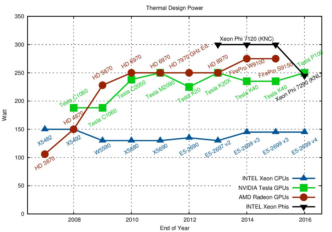
• GPUs have made finishing gradient descent in a reasonable amount of time possible.
• GTX 1080i is 10x faster than faster CPU and costs about 700,asopposedto4115.

From https://www.karlrupp.net/2013/06/cpu-gpu-and-mic-hardware-characteristics-over-time/

• Standard neural network do support the universal approximation theorum, they require an exponentially increasing number of parameters.
  • Solution: add multiple hidden layers to get super linear scaling. Enter: Deep Learning.

00:53:58 - Examples of Deep Learning applications¶

• Started investing in Deep Learning in 2012 (hired Geoffrey Hinton).
  • Now used in almost all Google products.
• Examples of Deep Learning in products:
  • Google Inbox recommending responses.
  • Skype translating language in real time.
• Paper: Semantic Style Transfer and Turning Two-Bit Doodles into Fine Artworks.
• Detecting cancer using CNNs.
• Lots of other examples (00:58:50).

00:59:14 - Understanding CNNs¶

• Key piece of CNN: convolution.
  • Great example of a single convolution: http://setosa.io/ev/image-kernels/
  • Basically, applying a filter over an image.
  • Neural network actually learns the most important set of filters for your problem.
  • Kernel size refers to the dimensions of the filter. In deep learning, it's usually 3x3.
• Add non-linear layer.
  • Non-linearity: takes an input value and turns it into some other value in a non-linear way.
    • Sigmoid.
    • Relu: most common type of activation.
      • Simply replaces negative values with 0: max(0, value)
• Need a way to set the parameters: stochastic gradient descent.
  • Basic idea to fit a function:
    1. Start with some point at random.
    2. Go a little bit to the left and to the right to find out which way is down.
    • In other words: you're calculating the derivative of the function at that point: dydx
    3. Now take a small step in the downwards direction by updating the guess as follows:
    Xn+1=Xn+dydx∗α
    • Need to ensure α aka the "learning rate" is a small enough number so you aren't jumping over the minima.
• What happens when you combine enough kernels, with enough layers and the SGD algorithm?

01:08:22 - Visualizing Convolutional Networks¶

• Paper by Matthew D. Zeiler: https://arxiv.org/abs/1311.2901
  • For each image, what are examples of filters that activate them?
  • Found that earlier layers tend to find things like shapes and textures.
  • By 3rd layer, started to find things like text, human faces.
  • By the 5th layer, able to recognise animals eyes, dog faces etc.

01:11:40 - Setting the learning rate¶

• Couple of numbers passed to the learn.fit method. The first is the learning rate.
  • How quickly should you walk toward the minima?
  • Setting the number well is very important:
    • too high = over step the minimia.
    • too low = takes too long to converge.
• Good idea for setting the learning rate from paper Cyclical Learning Rates for Training Neural Networks
  • Start by taking a tiny step in the gradient direction.
  • Then, take a slightly larger step.
  • Repeat until the loss gets worse.
  • Find the point where it's dropping the fastest.
• Plotting the learning rate against the loss:

• Learning rate scheduler is available in Fast.AI, as the lr_find method on a ConvLearner:

• You can plot the learning rate schedule using plot_lr():

• In that plotted example, the learning rate is increasing exponentially. It could also be increase linearly.
• We can call learn.sched.plot() to plot the loss verse learning rate (same plot as the gif above):

• We want the highest learning rate we can get, where the loss is clearly improving.
  • In this example, it's around 10−2

01:18:50 - Setting the num epochs¶

• Epoch = stepping through entire set of images.
• Answer to how many epochs: as many as you like.
  • After running a number of epochs, you might start to see accuracy decrease. When it decreases, you know you've run enough epochs.
  • Number of epochs can be based on the time you have available.

01:20:35 - Goals for the week¶

• Ensure you can run the 3 lines of code on the provided data and also on your own datasets.
• Get a sense of what's in the data object:
  • What do all the attributes and methods dos?
• Get familiar with NumPy.

01:21:51 - Jupyter notebook tricks¶

• If you can't remember how to spell, hit tab to get list of methods.
• To find the arguments to a method, use shift tab or ?, press it twice to get the docs.
• Prepend method with ?? to get source code.
• Press h to get keyboard shortcuts to Jupyter.
  • Students should try to learn 4 or 5 shortcuts a day.

01:25:20 - Closing notes¶

• Remember to shut off Paperspace (or Crestle) machine when done.
• Remember the forums if you get stuck.
• Make sure you read the info on course.fast.ai for each lesson.