Notes by Lex Toumbourou

This article is part of my (WIP) series on Reinforcement Learning.

Q-Learning is a reinforcement learning algorithm for finding optimal policies in Markov Decision Process. Unlike supervised learning, where we learn from labelled examples, Q-learning learns from interaction with an environment. It can learn the value of actions without requiring a model of the environment (i.e. learning via trial-and-error), hence, it is considered a "model-free" method.

The algorithm was introduced by Chris Watkins in his 1989 PhD thesis at King's College ¹, with a convergence proof later published by Watkins alongside Peter Dayan ². The concept was also developed independently by several others in the early 90s.

How It Works

Q-Learning is an iterative optimisation algorithm, similar to Gradient Descent in supervised learning. While gradient descent updates model parameters to minimise a loss function, Q-Learning refines value estimates based on environmental interaction. It utilises the Bellman Equation to update its predictions iteratively.

At the core is a lookup table called a Q-Table, which maps state-action pairs to expected future rewards. The values in the Q-Table are called Q-Values. Conceptually, a Q-value $Q(s,a)$ represents "how good" it is to take action a when in state s.

Rewards are discounted over time, meaning immediate rewards are valued more than distant ones – like how businesses value present cash flow over future earnings.

The algorithm uses three key hyper-parameters:

• Learning Rate $\alpha$ (0 to 1) – how quickly the algorithm updates its estimates. Higher values mean faster learning but potentially unstable convergence.
• Discount Factor $\gamma$ (0 to 1) – how much it values future rewards versus immediate ones. Higher values mean the agent is more forward-thinking.
• Exploration Rate $\epsilon$ (0 to 1) – how often it chooses a random action over the current best action. This parameter is typically decreased over time as the agent learns.

The $\epsilon$ parameter balances the trade-off between exploration and exploitation, managing how much the agent tries new things versus sticking to what it already thinks is best. See also the Exploration-Exploitation Dilemma in A/B testing.

Q-Learning in Practice: Taxi

We'll use the Taxi-v3 environment from the gymnasium library (formerly OpenAI Gym). In this environment, the agent (a taxi) must navigate a grid to pick up and drop off passengers at the right location.

Setup Code

You can install Gymnasium with the toy-text dependencies:

pip install "gymnasium[toy-text]"

Then run this code in a Python script:

import gymnasium as gym
import numpy as np
from gymnasium.wrappers import RecordVideo
from pathlib import Path
from tqdm import tqdm
import matplotlib.pyplot as plt

# Q-learning hyperparameters
alpha = 0.1      # Learning rate
gamma = 0.99     # Discount factor
epsilon = 0.1    # Exploration rate (probability of random action)

# An episode is a start-to-finish exploration of the state space,
# where the finish reaches a goal or a hazard.
episodes = 10_000

# Create the Taxi environment
env = gym.make("Taxi-v3", render_mode="human")

# Initialize Q-table with zeros
n_states, n_actions = env.observation_space.n, env.action_space.n
Q = np.zeros((n_states, n_actions))

# Training loop
for ep in tqdm(range(episodes), desc="Training episodes"):
    state, _ = env.reset()
    done = False
    total_reward = 0

    # Episode loop
    while not done:
        # Epsilon-greedy action selection
        if np.random.random() < epsilon:
            # Explore: random action
            action = env.action_space.sample()
        else:
            # Exploit: best known action
            action = np.argmax(Q[state])

        # Take action and observe new state and reward
        next_state, reward, terminated, truncated, _ = env.step(action)
        done = terminated or truncated
        total_reward += reward

        # Q-learning update using Bellman Equation
        # The temporal difference (TD) error represents how surprised we are by the outcome
        td_error = reward + gamma * np.max(Q[next_state]) - Q[state, action]
        Q[state, action] += alpha * td_error

        # Move to next state
        state = next_state

env.close()

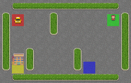
The code above will show a visual representation of the agent exploring and slowly updating its policy. Early episodes often show random-looking behaviour:

After training is completed, the final episodes demonstrate much more efficient behaviour:

As you can see, the taxi can pick the passengers up and drop them off at the destination directly.

Testing the Trained Policy

With a trained policy, we can use argmax to pick the highest reward action at every step, effectively using the policy without any more exploration:

# Test the learned policy
state, _ = env.reset()
env.render()
done = False
total_reward = 0

print("Testing trained policy...")
while not done:
    # Always choose the best action according to Q-table
    action = np.argmax(Q[state])
    state, reward, terminated, truncated, _ = env.step(action)
    total_reward += reward
    done = terminated or truncated
    print(f"Step reward: {reward}, Total reward: {total_reward}")
    print(env.render())

print(f"Final score: {total_reward}")

Q-Learning Update Rule: The Math Behind It

The core of the Q-Learning algorithm is its update rule, which is derived from the Bellman Equation. Let's break it down step by step:

$Q(s,a) \leftarrow Q(s,a) + \alpha \Big[ r + \gamma \max_{a'} Q(s', a') - Q(s,a) \Big]$

Where:

• $Q(s,a)$: Current estimate of value for taking action $a$ in state $s$
• $\alpha$: Learning rate (how quickly we update our estimates)
• $r$: Immediate reward received after taking the action
• $\gamma$: Discount factor (importance of future rewards)
• $s'$: The next state we arrive at
• $\max_{a'} Q(s', a')$: Value of the best possible action in the next state
• $\Big[ r + \gamma \max_{a'} Q(s', a') - Q(s,a) \Big]$: The temporal difference (TD) error

In simpler terms:

1. We take our current estimate $Q(s,a)$
2. Calculate the TD error (difference between ideal and current estimate)
3. Update our estimate by moving it slightly (by $\alpha$) toward the ideal

Deep Q-Learning

For complex environments with large state spaces, maintaining a Q-table becomes impractical or impossible. For example, in Atari games, where the state is a raw pixel image, there are millions of possible states.

In 2013, DeepMind published a landmark paper where they replaced the Q-table with a Neural Network to approximate the Q-values - a technique known as Deep-Q Learning or DQN ³.

The neural network inputs the state and outputs Q-values for all possible actions, which allows the algorithm to generalise across similar states and handle continuous state spaces.

See the Deep-Q Learning article for more.

Summary

Q-learning provides a fundamental approach to reinforcement learning by learning state-action values through interaction with an environment. Its simplicity and effectiveness make it a cornerstone algorithm in the field, while extensions like Deep Q-Learning enable its application to complex real-world problems.

Backlinks

• Markov Decision Process