A Discriminative Feature Learning Approach for Deep Face Recognition
These are my notes from the paper A Discriminative Feature Learning Approach for Deep Face Recognition by Yandong Wen, Kaipeng Zhang, Zhifeng Li, and Yu Qiao.
Abstract
We commonly train image classification models using Categorical Cross-Entropy Loss. However, softmax loss does not learn sufficiently discriminative features for face recognition.
This paper proposes a new supervision signal called Center Loss. Center Loss simultaneously learns a center for each class and penalizes the distance between features and their class centers.
Center Loss requires training with joint supervision of softmax loss for stability.
The paper improves on the state-of-the-art for face recognition and face verification tasks.
1. Introduction
Modern image classification typically involves some backbone model to learn features from input images, which we can feed into a final fully-connected layer for classification.
At the time of the paper, CNNs were the best-performing model architecture for learning features.
Since image classification problems are typically Close-Set (all possible test classes well represented in the training set), Categorical Cross-Entropy Loss table loss function choice. In this case, the features learned by the backbone model only need to be separable enough so the classifier can distinguish between classes.
However, in facial recognition, you cannot pre-collect all possible test identities in the training set for face recognition. We call these problems Open-Set Classification. Therefore, for facial recognition, we need to learn discriminative features.
Discriminative features have two properties:
- features from the same class should be close together, aka "inter-class dispensation."
- features from different classes should be far apart, aka "intra-class compactness."
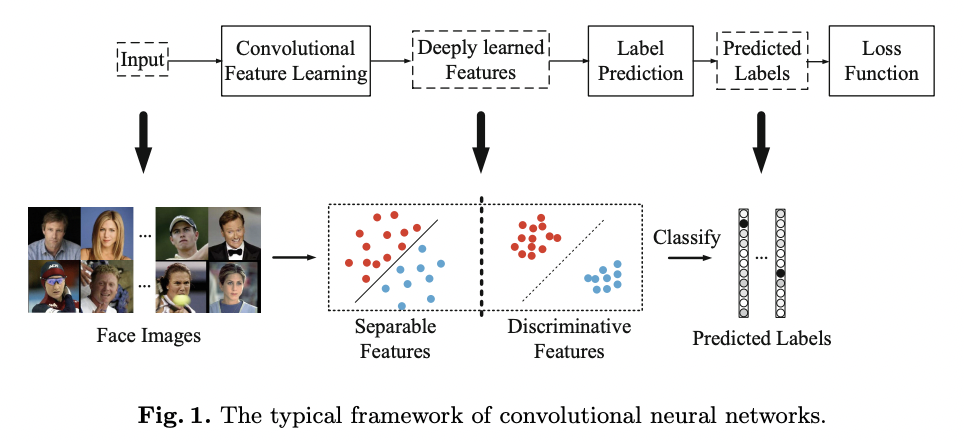
In Fig 1. we see a typical image classification pipeline, comparing separable and discriminative features.
Typically recognition pipelines use a Nearest Neighbours or K Nearest Neighbours step to classify faces based on the distance to other identities instead of label predictions.
Constructing a loss function for discriminative feature learning is challenging.
Since Stochastic Gradient Descent (SGD) relies on mini-batches, you cannot represent the global distribution in every step.
Alternatives proposed include Contrastive Loss (training using pairs) and Triplet Loss (training using triplets). However, they rely on Hard Negative Mining for efficiency, which adds complexity to the training pipeline.
This paper proposes Center Loss. They add a center for each class, a vector of the same dimension as the input feature embedding.
They simultaneously learn center during training while minimizing the distance between features and their corresponding class center.
The backbone requires trained using joint supervision of Categorical Cross-Entropy LossLoss, with a new hyperparameter to balance each component.
The center loss pulls deep features of the same class toward their centers, accomplishing the goal of inter-class compactness and intra-class dispersion.
Paper runs experiments on:
- MegaFace Challenge
- Labeled Faces in the Wild (LFW)
- YouTube Faces (YTF)
2. Related Work
- Face recognition with Deep Learning
- Parkhi, O.M., Vedaldi, A., Zisserman, A.: Deep face recognition. In: Proceedings of the British Machine Vision, vol. 1, no. 3, p. 6 (2015)
- Schroff, F., Kalenichenko, D., Philbin, J.: Facenet: a unified embedding for face recognition and clustering. In: Proceedings of the IEEE Conference on Computer Vision and Pattern Recognition, pp. 815–823 (2015)
- Sun, Y., Chen, Y., Wang, X., Tang, X.: Deep learning face representation by joint identification-verification. In: Advances in Neural Information Processing Systems, pp. 1988–1996 (2014)
- Sun, Y., Wang, X., Tang, X.: Hybrid deep learning for face verification. In: Proceedings of the IEEE International Conference on Computer Vision, pp. 1489–1496 (2013)
- Taigman, Y., Yang, M., Ranzato, M., Wolf, L.: Deepface: closing the gap to human level performance in face verification. In: Proceedings of the IEEE Conference on Computer Vision and Pattern Recognition, pp. 1701–1708 (2014)
- Wen, Y., Li, Z., Qiao, Y.: Latent factor guided convolutional neural networks for age-invariant face recognition. In: Proceedings of the IEEE Conference on Computer Vision and Pattern Recognition, pp. 4893–4901 (2016)
- Mapping pair of face images to distance
- Chopra, S., Hadsell, R., LeCun, Y.: Learning a similarity metric discriminatively, with application to face verification. In: 2005 IEEE Computer Society Conference on Computer Vision and Pattern Recognition, CVPR 2005, vol. 1, pp. 539–546. IEEE (2005).
- They train siamese networks to drive the similarity metric to be small for positive and large for negative pairs.
-
- Hu, J., Lu, J., Tan, Y.P.: Discriminative deep metric learning for face verification in the wild. In: Proceedings of the IEEE Conference on Computer Vision and Pattern Recognition, pp. 1875–1882 (2014)
- Introduce a margin between positive and negative face image pairs.
- Chopra, S., Hadsell, R., LeCun, Y.: Learning a similarity metric discriminatively, with application to face verification. In: 2005 IEEE Computer Society Conference on Computer Vision and Pattern Recognition, CVPR 2005, vol. 1, pp. 539–546. IEEE (2005).
- Softmax modifications
- Sun, Y., Wang, X., Tang, X.: Deep learning face representation from predicting 10,000 classes. In: Proceedings of the IEEE Conference on Computer Vision and Pattern Recognition, pp. 1891–1898 (2014)
- Taigman, Y., Yang, M., Ranzato, M., Wolf, L.: Deepface: closing the gap to human level performance in face verification. In: Proceedings of the IEEE Conference on Computer Vision and Pattern Recognition, pp. 1701–1708 (2014)
- Joint Identification Verification Supervision Signal
- Sun, Y., Chen, Y., Wang, X., Tang, X.: Deep learning face representation by joint identification-verification. In: Advances in Neural Information Processing Systems, pp. 1988–1996 (2014)
- Wen, Y., Li, Z., Qiao, Y.: Latent factor guided convolutional neural networks for age-invariant face recognition. In: Proceedings of the IEEE Conference on Computer Vision and Pattern Recognition, pp. 4893–4901 (2016)
- Sun, Y., Wang, X., Tang, X.: Deeply learned face representations are sparse, selective, and robust. In: Proceedings of the IEEE Conference on Computer Vision and Pattern Recognition, pp. 2892–2900 (2015)
- Add fully connected layer and loss functions to each conv layer.
- Triplet Loss
- Liu, J., Deng, Y., Huang, C.: Targeting ultimate accuracy: Face recognition via deep embedding. arXiv preprint (2015). arXiv:1506.07310
- Parkhi, O.M., Vedaldi, A., Zisserman, A.: Deep face recognition. In: Proceedings of the British Machine Vision, vol. 1, no. 3, p. 6 (2015)
- Schroff, F., Kalenichenko, D., Philbin, J.: Facenet: a unified embedding for face recognition and clustering. In: Proceedings of the IEEE Conference on Computer Vision and Pattern Recognition, pp. 815–823 (2015)
- In this paper, they minimise the distance between an anchor and a positive, while maximising the distance between an anchor and a negative until the margin is met.
3. The Proposed Approach
The authors use a toy example to intuitively show the distribution of deeply learned features. Inspired by this distribution, they propose center loss to improve the discriminative power of the learned features.
The toy example is trained on MNIST. They modify LeNet (a standard convolutional architecture) to include an extra conv layer (making up three conv layers in total) and additional conv filters in each layer. Then they reduce the output of the last hidden layer to 2, so they can visualize features in 2d space.
Fig 2. shows the results of plotting the 2-dimension hidden layer output on the training set (a) and the test set (b).
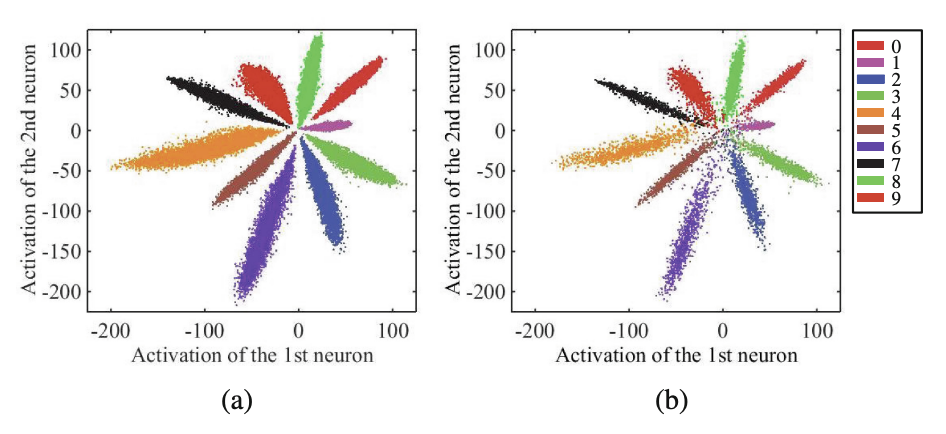
We can infer from this that the learned features are separable - a classifier can find a decision boundary between them - but not discriminative. In other words, it would be challenging to classify features using the nearest neighbors approach, as the distance between intra-class samples often matches those inter-class.
Center loss function is proposed to address this:
Where:
- refers to the size of the mini-batch
- refers to the th class center of the deep features.
Since we cannot take the entire training set into account to average features of every class in each iteration, we have to make two modifications to support mini-batches.
- Centers are computed by averaging features of the corresponding class (some centers may not update in a mini-batch)
- Control the learning rate of the center using param to avoid mislabelled samples breaking everything.
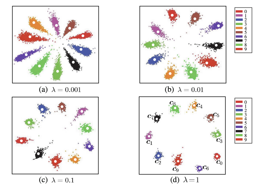
Lastly, they train the model using joint supervision of softmax loss and center loss, using hyperparameters . When , training uses conventional Softmax Loss.
Fig 3. shows how the hyperparameters affect the feature distributions. The higher it is, the more discriminative the features.

Joint supervision is necessary: if you only trained using class centers, the centers would degrade to 0 since that creates the lowest possible center loss.
The method is superior to contrastive and triplet loss as it is efficient and easy to implement.
4. Experiments
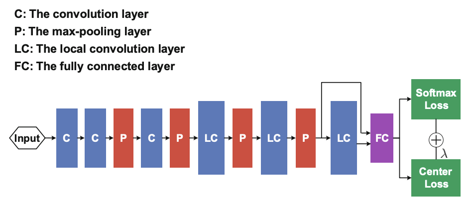
They use a typically CNN archiecture for the experiments.
Filter sizes for conv and local conv layers are 3x3 with stride 1, followed by PReLU nonlinear units.
The number of feature maps is 128 for conv layers and 256 for local conv layers. Max-pooling grid is 2x2, and the stride is 2.
They concatenate the output of the 4th pooling layer and the 3rd local conv layer as input to the 1st fully connected layer. The output of the fully connected layer is 512.
In Fig 4, we see a diagram of this architecture.
4.1 Implementation Details
Use five landmarks (2 eyes, nose, and mouth corners) for similarity transformation.
When detection fails, discard the image in the training set, but use the provided landmarks if it is a testing image.
Faces are cropped to 112 x 96 RGB images.
Each pixel is normalized by subtracting 127.5 and dividing by 128.
Training data uses web-collected training data, including:
- CASIA-WebFace
- CACD2000
- Celebrity
They remove images with identities appearing in testing datasets, which goes to 0.7M images of 17,189 unique persons.
The authors horizontally flip images for augmentation.
They train three types of models for comparison:
- Model A: Softmax loss
- Model B: Softmax and contrastive loss
- Model C: Softmax and center loss
They extract features for each image and the horizontally flipped one and concatenate them as representation.
They compute the score as Cosine Distance of 2 features after PCA.
They use Nearest neighbor and threshold comparison for Face Identification and Face Verification tasks.
4.2 Experiments on the Parameter and
They conducted experiments to investigate the sensitivity of the params on Labeled Faces in the Wild dataset.
The results are shown in Fig 5, for 2 experiments:
Experiment (a)
- Fix to 0.5.
- Vary from 0 to 0.1 to train different models.
Experiment (b)
- Fix
- Vary from 0.01 to 1.
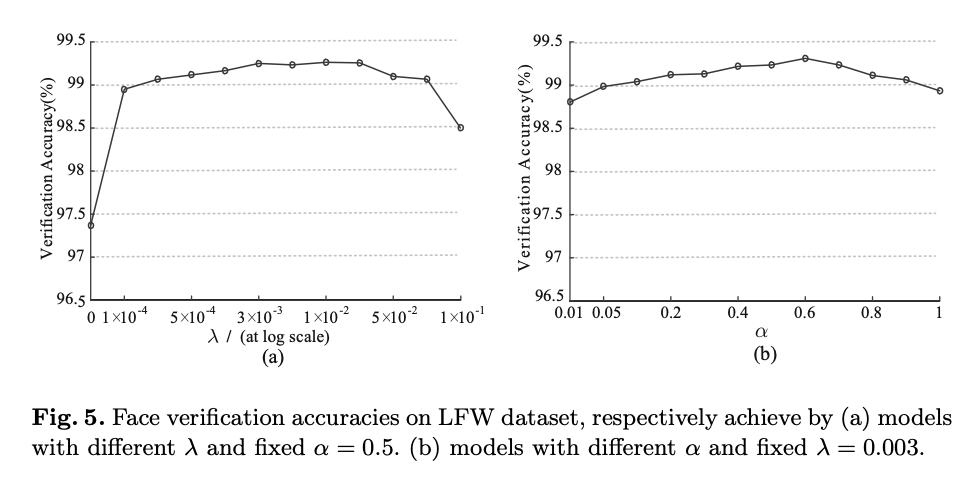
From this they infer:
- Softmax Loss alone is not a good choice. It leads to poor verification performance.
- Properly choosing a value of can improve verification accuracy.
- Verification performance of model remains stable across a range of and .
4.3 Experiments on the LFW and YTF Datasets
Evaluate single model on Labeled Faces in the Wild and YouTube Faces.
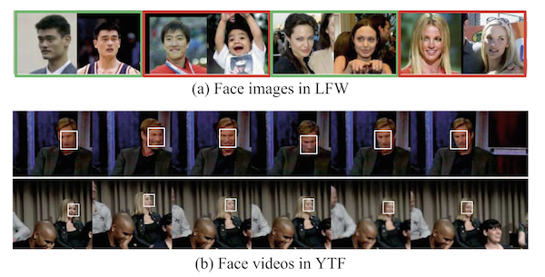
Fig 6. has some examples.
In (a), they show pairs in LFW the green frame is for positive pairs, and the red frame is for negative ones.
In (b), they show examples from YTF, where the white bounding box is the face for testing.
They train model on only 0.7M outside data with no overlapping in LFW and YTF. Fix and for Model C.
LFW dataset contains 13,233 web-collected images from 5749 identities, with variations in pose, expression, and illuminations. They test on 6,000 face pairs and report the experiment results.
YTF dataset consists of 3,425 videos of 1,595 different people, with an average of 2.15 videos per person. The clip durations vary from 48 to 6,070 frames, with an average length of 181.3 frames.
Table 2 has the results on 5,000 video pairs.
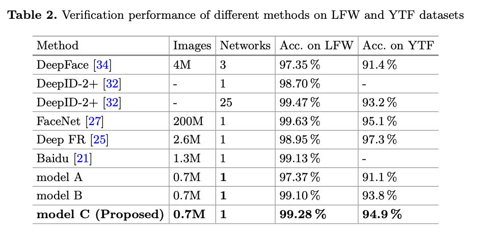
They observe the following:
- Softmax Loss and Center Loss beats baseline one (Model A) by a large margin.
- Joint supervision can notably enhance the discriminative power of deeply learned features, demonstrating the effectiveness of center loss over Softmax.
- It also improves over Softmax and Contrastive Loss.
- Using less training data and simpler architectures, they outperform many state-of-the-art approaches.
4.4 Experiments on MegaFace Challenge Dataset
MegaFace datasets aim to evaluate the performance of face recognition algorithms with millions of distractors (people who are not in the testing set).
MegaFace dataset has two parts:
- Gallery Set. 1 million images from 690K people. A subset of Flickr photos from Yahoo.
- Probe Set. It consists of 2 datasets:
- Facescrub contains 100K photos of 530 unique people.
- FGNet. Face Aging Dataset, with 1002 images from 82 identities. Each identity has multiple face images at different ages (ranging from 0 to 69).
The challenge has several testing scenarios: Identification, Verification, and Pose Invariance with two protocols: large or small training set.
The Center Loss authors follow a small training set protocol, which is less than 0.5M images and 20K subjects. They reduced the size of the training image dataset to 0.49M but kept the number of identities unchanged at 17,189.
They discard any images overlapping with Facescrub dataset.
They train three models: Model A, B, and C for comparison.
They use the same settings as earlier the is 0.003 and the is 0.5 in Model C.
They test the algorithm on only one of the three galleries.
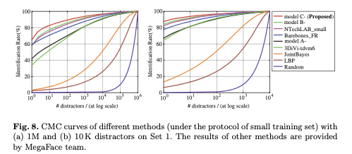
Face Identification
Face identification aims to match a given probe image to those with the same person in the gallery. This task computes the similarity between each given probe face image and the gallery, including at least one image with the same identity as the probe one. The gallery contains a different scale of distractors, from 10 to 1 million, leading to increasing testing challenges.
In Fig 8, they show the results of face identification experiments. They measure performance using Cumulative Match Characteristics (CMC) curves, which is the probability that a correct gallery image is in top-K.
Face Verification
For face verification, the algorithm should decide whether a given pair of images is the same person or not.
They create four billion negative pairs between the probe and gallery datasets.
They compute the True Accept Rate (TAR) and False Accept Rate (FAR) and plot the Receiver Operating Characteristic (ROC) curves of different methods in Fig. 9.
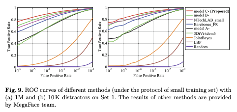
Some of the methods they compare against include methods that require hand-crafted features, including LBP (Local Binary Pattern) and shallow models like JointBayes.
From Fig. 8 and Fig. 9, we can see that these modes perform poorly: their accuracies drop as the number of distractors increases.
Model C performs the best out of A and B and outperforms the other published methods.
To be practical, face recognition models should achieve high performance with millions of distractors.
Table 3 reports the rank-1 identification rate with at least 1 million distractors.
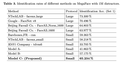
Table 4 reports the True Accept Rate with a False Accept Rate of .
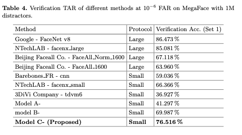
They make these observations from the results:
- Model C is much better than Model A and Model B for face identification and verification tasks, confirming Center Loss with Softmax works best.
- Second, under the evaluation protocol of a small training set, the proposed Model C- achieves the best results in both face identification and verification tasks, outperforming 2nd place by 5.97% on face identification and 10.15% on face verification, respectively.
- Model C does better than some models trained with a large training set (e.g., Beijing Facecall Co.).
- The models from Google and NTechLAB achieve the best performance thanks to the large training set (500M vs. 0.49M).
5 Conclusions
The paper proposes a new loss function called Center Loss.
By combining Center Loss with Softmax Loss to jointly supervise the learning of CNNs, the authors show that they can enhance the discriminative power of features for face recognition problems.
The paper runs extensive experiments on large-scale face benchmarks to demonstrate its effectiveness.