Eigenvectors and Eigenvalues
These are notes from Eigenvectors and eigenvalues | Chapter 14, Essence of linear algebra by Khan Academy.
Consider a linear transformation in 2d, . Most vectors don't continue along their span after the transformation.
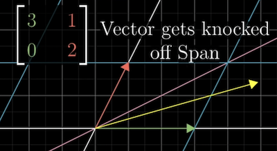
However, some particular vectors do remain on their span. The vector moves over to 3x itself but still on the x-axis.
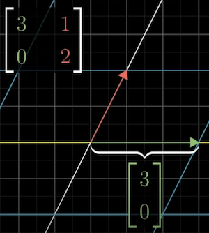
Because of how linear transformations work, any other vector on the same axis is scaled by 3.
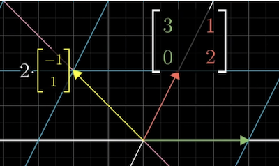
Another vector also stays on its span during the transformation. It is stretched by a factor of 2, as does any vector on the same span.
These vectors are called the Eigenvectors.
Each Eigenvector has an associated Eigenvalue. The Eigenvalue refers to how it stretches or squishes the Eigenvector during the transformation.
The Eigenvalues can be negative and fractional.
Finding Eigenvectors is useful in 3d transformations because the Eigenvector is the axis of rotation.
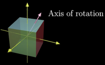
It is much easier to think about a 3d rotation using the axis of rotation and the angle it's rotating, rather than thinking of the 3x3 matrix that describes the rotation.
The Eigenvalue here must be one since rotations don't stretch or squish anything.
Sometimes a way to understand a transformation is to find the Eigenvectors and Eigenvalues.
Symbolically, an Eigenvector is described like this:
Where: * is the matrix representing a transformation. * is the Eigenvector. * is a number representing the Eigenvalue.
The expression is saying: the Matrix-vector product is the same as scaling the Vector by .
So finding the Eigenvalues and Eigenvectors of is about finding the value and that make the expression true.
It's a bit strange to have matrix multiplication on one side and scalar multiplication on the other side, so we can rewrite it using the identity matrix as follows:
We can then subtract off the right-hand side:
Then factor out the :
If is 0, that will satisfy the answer, but you want a non-zero as an Eigenvector.
From the lesson on Matrix Determinate, we know that the only way the transformation of a matrix with a non-zero vector is if transformation associated with that matrix squishes space onto a lower dimension. That corresponds to a 0 determinate for the matrix.
You can think about the determinate of this matrix:
If you had a value that was subtracting off each diagonal entry:
What lambda value would you need to get a 0 determinate? In this case, it happens when
So there's some vector when multiplied by equals 0.
Another example: to find out if a value is an Eigenvalue, subtract it from the diagonal and compute the determinate.
Doing that, gives you a quadratic polynomial in :
We know that the can only be an Eigenvalue if the determinate is 0; we can conclude that the only possible values for are 3 and 2.
To find the Eigenvectors that have these values, plug in the value to the matrix and solve to find which vectors return 0.
Some 2d transformations have no Eigenvectors (what about 3d transformations?). For example, a rotation transformation takes all vectors of their span.
If we try to calculate the determinate: , the only possible solution is for to be imaginary number or . Having no real number solutions tells us there aren't any Eigenvectors.
A shear is another interesting example. It fixes in place and makes . All vectors on x-axis are Eigenvectors with Eigenvalues of 1.
When you calc the determinate, , you get . The only root of the expression is .
It's possible to have one Eigenvalue with multiple Eigenvectors. A matrix that scales everything by 2: makes every vector in the plane an Eigenvector, with the only Eigenvalue being 2.
What happens if both basis vectors are Eigenvectors? One example is .
Notice how there's a positive value on the diagonal and 0s everywhere else? That's a Diagonal Matrix.
The way to interpret it is that all the basis vectors are Eigenvectors, with the diagonal entry being Eigenvalues.
There are a lot of things that make diagonal matrices much easier. One of them is that it's easy to reason about what happens when you apply the matrix multiple times. You are simply multiplying the diagonal values multiple times.
Contrast that with normal matrix multiplication. It quickly gets complicated.
The basis vectors are rarely Eigenvectors. But if your transformation has at least 2 Eigenvectors that span space, you can change your coordinate system so that your Eigenvectors are your basis vectors by Changing Basis. The composed matrix will be Diagonal Matrix.
So, if you need to compute the 100th power of a matrix, it's easier to first convert to an Eigenbasis. Perform the computation. Then convert back to the original basis.
Note that not all transformations will support this. Shear or rotation don't have enough Eigenvectors to support this, for example.