Notes by Lex Toumbourou

Matrices make linear mappings

Matrices as objects that map one vector onto another; all the types of matrices

Introduction: Einstein summation convention and the Symmetry of the dot product

• Einstein Summation Convention (00:00-04:24)

  • We can represent a Matrix Multiplication between matrix $A$ and matrix $B$ like this:

    $\begin{bmatrix}a_{11} & a_{12} & a_{13} \\ a_{21} & a_{22} & a_{23} \\ a_{31} & a_{32} & a_{33}\end{bmatrix} \begin{bmatrix}b_{11} & b_{12} & b_{13} \\ b_{21} & b_{22} & b_{23} \\ b_{31} & b_{32} & b_{33}\end{bmatrix} = AB$

    We can think of one of the elements in row 2, column 3 of $AB$ as:

    ${(ab)}_{23} = a_{21}b_{13} + a_{22}b_{23} + a_{23}b_{33}$

    We can rewrite that as the sum of elements $j$:

    $ab_{ik} = \sum\limits_{j} a_{ij} \cdot b_{jk}$

    In Einstein's convention, if you have a repeated index like $j$ you can remove it alongside the Sigma notation:

    $ab_{ik} = a_{ij} \cdot b_{jk}$

    The Einstein Summation Convention also describes a way to code Matrix Multiplication.

• Matrix Multiplication with rectangular matrices (04:24-05:55)

  • We can multiply rectangular matrices as long as the columns in the first are equal to the rows in the 2nd.

    $A_{(2 \times 3)} \cdot B_{(3 \times 4)}$

    The Einstein Summation Convention shows those operations work. As long as both matrices have the same number of $j$s, you can do it.

    $C_{ik} = a_{ij}b_{jk}$

• Dot Product revisited using Einstein's Summation Convention (05:55-07:14)

  • The dot product between vectors $\vec{u}$ and $\vec{v}$ in the summation convention is: $u_{i}v_{i}$

  • We can also consider a dot product a matrix product of a row vector and a column vector:

    

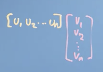
    So there's some equivalence between Matrix Multiplication and the Dot Product.

• Symmetry of the Dot Product (07:15-09:32)

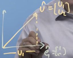
  • If we have unit vector $\hat{u} = \begin{bmatrix}u_1 \\ u_2\end{bmatrix}$ and we do a projection onto one of the axis vectors: $\hat{e_1} = \begin{bmatrix}1 \\ 0\end{bmatrix}$, we get a length of $u_1$

    

    • If we then project $e_1$ onto $\hat{u}$, we can draw a line of Symmetry between where the two projections cross:

      

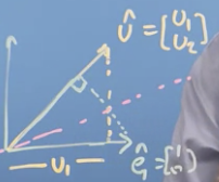
      • The two triangles on either side are the same size, proving that the projection is the same length in either direction. So that proves the Dot Product is symmetrical and also that projection is the Dot Product.
        • That explains why matrix multiplication with a vector is considered a projection onto the vectors composing the matrix (the matrix columns).

Matrics transform into the new basis vector set

Matrics changing basis

• Transforming a Vector between Basis Vectors (00:00-08:31)

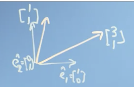
  • We can think of the columns of a transformation matrix, as the axes of the new basis vectors described in our coordinate system.
    • Then, how do we transform a vector from one set of basis vectors to another?

  • If we have 2 basis vectors that describe the world of Panda bear in at $\begin{bmatrix}3 \\ 1\end{bmatrix}$ and $\begin{bmatrix}1 \\ 1\end{bmatrix}$. Noting that these vectors are describes in the normal coordinate system with basis vectors $\begin{bmatrix}0 \\ 1\end{bmatrix}$ and $\begin{bmatrix}1 \\ 0\end{bmatrix}$

    

    • In Panda's world, those basis vectors are $\begin{bmatrix}1 \\ 0\end{bmatrix}$ and $\begin{bmatrix}0 \\ 1\end{bmatrix}$
      • If we have a vector described in Panda's world as $\frac{1}{2} \begin{bmatrix}3 \\ 1\end{bmatrix}$, we can get it in our frame, by multiplying with Panda's basis vectors: $\begin{bmatrix}3 & 1 \\ 1 & 1\end{bmatrix} \begin{bmatrix}\frac{3}{2} \\ \frac{1}{2} \end{bmatrix} = \begin{bmatrix}5 \\ 2 \end{bmatrix}$
    • Which begs the question: how can we translate between Panda's world into our world?
      • Using the Matrix Inverse of Panda's basis vector matrix we can get our basis in Bear's world:

    $B^{-1} = \frac{1}{2} \begin{bmatrix}1 & -1 \\ -1 & 3\end{bmatrix}$

    • If we use that to transform the vector in our world, we should get it in Bear's world.

      $\frac{1}{2} \begin{bmatrix}1 & -1 \\ -1 & 3\end{bmatrix} \begin{bmatrix}5 \\ 2\end{bmatrix} = \begin{bmatrix}\frac{3}{2} \\ \frac{1}{2}\end{bmatrix}$

• Translate between basis vectors using projections (08:32-11:14)

  • If the new basis vectors are orthogonal then we can translate between bases using only the dot product.

Doing a transformation in a changed basis

• Doing a transformation of a Vector in a changed basis (00:00-04:13)

  • How would you do a 45° rotation in Panda's basis?

  • You could first do it in a normal basis.

    $\frac{1}{\sqrt{2}} \begin{bmatrix}1 & -1 \\ 1 & 1\end{bmatrix}$

  • And multiply that by the vector in our basis:

    $\frac{1}{\sqrt{2}} \begin{bmatrix}1 & -1 \\ 1 & 1\end{bmatrix} \begin{bmatrix}3 & 1 \\ 1 & 1\end{bmatrix} \begin{bmatrix}x \\ y\end{bmatrix}$

  • That gives us the transformation in our basis vector. You can then multiply that by the inverse of the coordinate matrix, to get it in Panda's coordinate system.

    $\frac{1}{2} \begin{bmatrix}1 & -1 \\ -1 & 3\end{bmatrix} \frac{1}{\sqrt{2}} \begin{bmatrix}1 & -1 \\ 1 & 1\end{bmatrix} \begin{bmatrix}3 & 1 \\ 1 & 1\end{bmatrix} \begin{bmatrix}x \\ y\end{bmatrix}$

  • In short: $B^{-1} R B = R_{b}$

Making Multiple Mappings, deciding if these are reversible

Orthogonal matrices

• Matrix Transpose (00:15-01:08)
  • An operation where we interchange the rows and columns of a matrix.
  • ${A^{T}}_{ij} = A_{ji}$
  • $\begin{bmatrix}1 & 2 \\ 3 & 4\end{bmatrix}^{T} = \begin{bmatrix}1 & 3 \\ 2 & 4\end{bmatrix}$
• Orthonormal Basis Set (01:09-06:35)
  • If you have a square matrix with vectors that are basis vectors in new space, with the condition that the vectors are orthogonal to each other and they're unit length (1)
    • In math: $a_i \cdot a_j = 0, i \neq j$ $a_i \cdot a_j = 1, i = k$
    • When you multiple one of these matrices by their transpose, the identity matrix is returned.
      • That means $A^{T}$ is a valid identity for these examples.
    • A matrix composed of these is called Orthogonal Matrix.
    • The transpose of these matrices is another orthogonal matrix.
    • The determinant of these is 1 or -1.
    • In Data Science, we want an orthonormal basis set where ever possible.

Recognising mapping matrices and applying these to data

The Gram-Schmidt process

• Gram-Schmidt Process (00:00-06:07)
  • If you have vector set $v = {v_1, v_2 ... v_n}$ that span your space and are linear independent (don't have a determinate of 0) but aren't orthogonal or unit length, you can convert them into an Orthonormal Basis Set using the Gram-Schmidt Process.
  • Process:
    • Take the first vector in the set, $v_1$ and normalise so it's of unit length giving you $e_1$ the first basis vector: $e_1 = \frac{v_1}{|v_1|}$

    • We can think of $v_2$ as having a component in the direction of $e_1$ and a component that's perpendicular.

      

      • We can find the component in the direction of $e_1$ by finding the vector projection of $v_2$ onto $e_1$: $\frac{v_2 \cdot e_1}{|e_1|}$
        • To get as a vector we multiply by $e_1$ (noting that it's already of unit length): $\frac{v_2 \cdot e_1}{|e_1|} e_1$
        • We know that $v_2$ is equal to that + the perpendicular component: $v_2 = \frac{v_2 \cdot e_1}{|e_1|} e_1 + u_2$
        • We can rearrange the expression to find $u_2$: $u_2 = v_2 - (v_2 \cdot e_1) e_1$
        • If we normalise $u_2$: $\frac{u_2}{|u_2|}$ the result is $e_2$
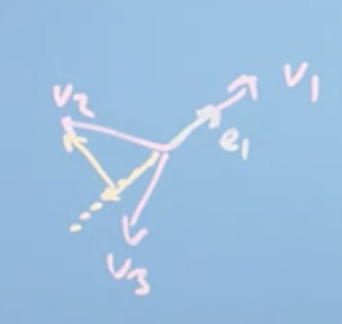
          • Now to find $e_3$, which we know isn't a linear combination of $e_1$ and $e_2$:
      • We can project is onto the plane of $e_1$ and $e_2$, which will result in a vector in the plane composed of $e_2$ and $e_1$s.
      • We can then find the components of $v_3$ that aren't made up of $v_1$ and $v_2$:
        • $u_3 = v_3 - (v_3 \cdot e_1)e_1 - (v_3 \cdot e_2)e_2$
        • If we normalise $u_3$, we get $e_3$: $e_3 = \frac{u_3}{|u_3|}$ we have another unit vector that's normal to the plane.
          • We can keep doing this through all $v_n$ until we have basis vectors that span the space.

Example: Reflecting in a plane

• Example: performing a rotation on a vector with an unfamilar plane.
  • Create Orthogonal Matrix plane with Gram-Schmidt Process.
• Challenge: performing a rotation on a vector with an unfamiliar plane.
  • You know 2 vectors in the space: $\begin{bmatrix}1 \\ 1 \\ 1\end{bmatrix}$ and $\begin{bmatrix}2 \\ 0 \\ 1\end{bmatrix}$
  • You have a 3rd vector out of the mirror's plane: $\begin{bmatrix}3 \\ 1 \\ -1\end{bmatrix}$
  • First part, find basis vectors:
    • Find $e_1$: normalise $v_1$ to find $e_1$: $e_1 = \frac{v_1}{|v_1|} = \frac{1}{\sqrt{3}} \begin{bmatrix}1 \\ 1 \\ 1 \end{bmatrix}$
    • Then $e_2$, starts with $u_2$: $u_2 = v_2 - (v_{2} \cdot e_{1}) * e_{1}$ then normalise that.
    • Lastly, $e_3$: is the normalised: $u_3 = v_3 - (v_{3} \cdot e_{1}) e_{1} - (v_{3} \cdot e_{2}) e_{2}$
    • Result is a transformation matrix described by the basis refactors: $E = \begin{bmatrix}(e_1) & (e_2) & (e_3) \end{bmatrix} = \left(\frac{1}{\sqrt{3}} \begin{bmatrix}1 \\ 1 \\ 1 \end{bmatrix} \frac{1}{\sqrt{2}} \begin{bmatrix}1 \\ -1 \\ 0\end{bmatrix} \frac{1}{\sqrt{6}} \begin{bmatrix}1 \\ 1 \\ -2 \end{bmatrix} \right)$
    • We can rotate a vector by 45° in a single plane, we can flip only the third column vector: $T_{E} = \begin{bmatrix}1 & 0 & 0 \\ 0 & 1 & 0 \\ 0 & 0 & -1\end{bmatrix}$
  • Now, we need to use this to convert a vector $r$ and want to apply to a transformation matrix but in a different space to make: $r'$
    • Going from $r$ to $r'$ is hard.

    • But if you first convert $r$ into the $e$ basis, then apply transformation and convert back into $r$, it's easy:

      

      • $E T_{E} E^{-1} r = r'$
        • Because $e$ is orthonormal, we know the transpose is the inverse.